Page 526 - Mechanical Engineers' Handbook (Volume 2)

5 Root Locus 517

G ( j ) dB G( j ) dB
1
1
/ G ( j ) G( j )
/
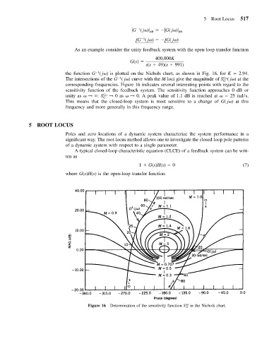
As an example consider the unity feedback system with the open-loop transfer function
400,000K
G(s)
s(s 49)(s 991)
1
the function G ( j ) is plotted on the Nichols chart, as shown in Fig. 16, for K 2.94.
1
The intersections of the G ( j ) curve with the M loci give the magnitude of S ( j ) at the
G cl
G
corresponding frequencies. Figure 16 indicates several interesting points with regard to the
sensitivity function of the feedback system. The sensitivity function approaches 0 dB or
unity as → : S G cl → 0as → 0. A peak value of 1.1 dB is reached at 25 rad/s.
G
This means that the closed-loop system is most sensitive to a change of G( j ) at this
frequency and more generally in this frequency range.
5 ROOT LOCUS
Poles and zero locations of a dynamic system characterize the system performance in a
significant way. The root-locus method allows one to investigate the closed-loop pole patterns
of a dynamic system with respect to a single parameter.
A typical closed-loop characteristic equation (CLCE) of a feedback system can be writ-
ten as
1 G(s)H(s) 0 (7)
where G(s)H(s) is the open-loop transfer function.

M in the Nichols chart.
Figure 16 Determination of the sensitivity function S G