Page 536 - Mechanical Engineers' Handbook (Volume 2)

5 Root Locus 527

at those locations by appropriate compensation. Compensation can be provided by introduc-
ing additional dynamics into the feedback system in the form of increased poles and zeros
[proportional-integral-derivative (PID) control, lead, lag, lead–lag, etc.]. We shall now con-
sider some examples to illustrate this time-domain design philosophy.

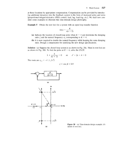
Example 5 Obtain the root loci for a system with an open-loop transfer function
K
G(s)
s(s 2)
(a) Indicate the location of closed-loop poles when K 4 and determine the damping
ratio
and the natural frequency corresponding to K 4.
n
(b) It is now required to double the natural frequency while keeping the same damping
ratio. Design a compensator for satisfying the new design specifications.

Solution: (a) Suppose the closed-loop system is as shown in Fig. 20a. Then its root loci are
as shown in Fig. 20b. To find the poles at K 4, solve the CLCE
4
1 0 or s 2s 4 0
2
s(s 2)
l j 3.
The roots are s 1,2

cos 0.5

Figure 20 (a) Time-domain design example; (b)
sketch of root loci.