Page 538 - Mechanical Engineers' Handbook (Volume 2)

5 Root Locus 529

Figure 22 Root loci with pole–zero cancella-
tion.

1. All the poles of the open-loop transfer function are in the closed left-half s-plane.
2. When the closed-loop system is excited by the input r(t) tu (t), the trace of Fig.
s
24b is obtained ( e 0).
1
3. When the gain K is doubled, the impulse response of Fig. 24c is observed.
Determine K, , and .

Solution: Since the closed-loop system has a finite steady-state error e for a ramp
1
input, the system should be type I. Thus we require either or to be zero. Let 0. So
it only remains to determine and K.
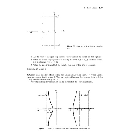
Now the root loci for the system can be sketched in the following manner.

Figure 23 Effect of nonexact pole–zero cancellation on the root loci.