Page 537 - Mechanical Engineers' Handbook (Volume 2)

528 Control System Performance Modification

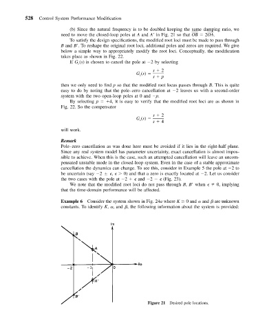
(b) Since the natural frequency is to be doubled keeping the same damping ratio, we
need to move the closed-loop poles at A and A in Fig. 21 so that OB 2OA.
To satisfy the design specifications, the modified root loci must be made to pass through
B and B . To reshape the original root loci, additional poles and zeros are required. We give
below a simple way to appropriately modify the root loci. Conceptually, the modification
takes place as shown in Fig. 22.
If G (s) is chosen to cancel the pole at 2 by selecting
c
s 2
G (s)
c
s p
then we only need to find p so that the modified root locus passes through B. This is quite
easy to do by noting that the pole–zero cancellation at 2 leaves us with a second-order
system with the two open-loop poles at 0 and p.
By selecting p 4, it is easy to verify that the modified root loci are as shown in
Fig. 22. So the compensator

s 2
G (s)
c
s 4
will work.
Remark
Pole–zero cancellation as was done here must be avoided if it lies in the right-half plane.
Since any real system model has parameter uncertainty, exact cancellation is almost impos-
sible to achieve. When this is the case, such an attempted cancellation will leave an uncom-
pensated unstable mode in the closed-loop system. Even in the case of a stable approximate
cancellation the dynamics can change. To see this, consider in Example 5 the pole at 2to
be uncertain (say 2 , 0) and that a zero is exactly located at 2. Let us consider
the two cases with the pole at 2 and 2 (Fig. 23).
We note that the modified root loci do not pass through B, B when 0, implying
that the time-domain performance will be affected.

Example 6 Consider the system shown in Fig. 24a where K 0 and and are unknown
constants. To identify K, , and , the following information about the system is provided:

Figure 21 Desired pole locations.