Page 644 - Mechanical Engineers' Handbook (Volume 2)

3 Frequency Compensation to Improve Overall Performance 635

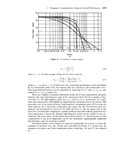
Figure 13 (Continued)(c) phase margin.

s 1
G c1 cz (16)
s 1
cp
where . For the example of Fig. 6b, the form would be
1
cz
s / (2 / )s 1
2
2
G c2 cz cz cz (17)
2
s / 2 (2 / )s 1
cp cp cp
where and . In both cases, the closed-loop performance is now determined
cz
2
cz
2
by the compensator poles since the original poles are canceled by the compensator zeros.
This augmented performance can be quantified by using Figs. 8–13, with , , sub-
cp
cp
cp
stituted for , , , respectively.
2
1
2
There are a number of practical limitations on the use of lead compensation, primarily
related to the large high-frequency gain of the compensator itself. For the examples of Eqs.
2
(16) and (17), the high-frequency gains are / and ( / ) , respectively. As a mini-
cz
cp
cp
cz
mum, this characteristic will amplify any high-frequency electrical noise in the system. With
reasonable care in the electrical design, high-frequency compensator gains of 10 or more are
often practical. For a first-order compensator, this means that the forward-loop break fre-
quencies can be boosted by a factor of 10, while the boost is only the square root of this
factor for a second-order compensator. Another problem associated with the gain boost of a
lead compensator is that poorly damped high-frequency modes can be excited or even de-
stabilized. This latter effect will be further discussed in Section 3.3. The practicality of lead
compensation in any given application can be best determined experimentally (additional
high-frequency lags are sometimes needed).
The high-frequency noise situation is improved considerably for systems in which the
integrator is electronic (e.g., the velocity servo described in Section 2.1). In this case, the
integrator can replace one of the compensator poles so that Eqs. (16) and (17) are replaced
by