Page 146 - Mechanics Analysis Composite Materials

Chapter 4. Mechanics of a composite layer 131

Indeed, consider a uniaxial tension as in Fig. 1.1 with stress 611. For this case,
a = and Eqs. (4.25) yield
CY = -+ o(o,)a., , (4.29)
01-
E
V 1
cy = --av - -o(a,)a., , (4.30)
E. 2
y.Yv = 0 .

Solving Eq. (4.29) for co(ax),we get
1 1
o(a.,) =--- , (4.31)
Es(0.r) E
where E, = is the secant modulus introduced in Section 1.1 (see Fig. 1.4).
Using now the existence of the universal diagram for stress intensity r~ and taking
into account that cr = a.,for a uniaxial tension, we can generalize Eq. (4.31) and
write it for an arbitrary state of stress as

(4.32)

To determine E,(o)= a/E, we need to plot the universal stress-strain curve. For this
purpose, we can use an experimental diagram o,(c,) for the case of uniaxial tension,
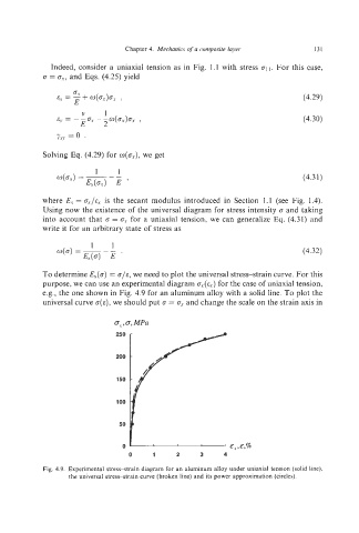
e.g., the one shown in Fig. 4.9 for an aluminum alloy with a solid line. To plot the
universal curve o(E),we should put 6 = a, and change the scale on the strain axis in

0,,6,MPU
250

200

150

100

50

0
0 1 2 3 4

Fig. 4.9. Experimental stress-strain diagram for an aluminum alloy under uniaxial tension (solid line),
the universal stress-strain curve (broken line) and its power approximation (circles).