Page 338 - Mechanics Analysis Composite Materials

Chapter 7. Environmenral,special loading, and manufacturing eiffects 323

2

1.8

1.6
1A

1.2

1 Days (24 Hours)
0 50 100 150
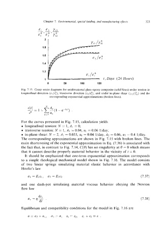
Fig. 7. IS. Creep strain diagrams for unidirectional glass-epoxy composite (solid lines) under tension in
longitudinal direction (E, /E:), transverse direction (EZ/E!)). and under in-plane shear and the
correspondingexponential approximations(broken lines).

For the curves presented in Fig. 7.15, calculation yields
longitudinal tension: N = 1, A1 = 0;
transverse tension: N = 1, AI = 0.04,cq = 0.06 l/day;
in-plane shear: N = 2, AI = 0.033, UI = 0.04 I/day, A? = 0.06, a2 = 0.4 l/day.
The corresponding approximations are shown in Fig. 7.15 with broken lines. The
main shortcoming of the exponential approximation in Eq. (7.36) is associated with
the fact that, in contrast to Fig. 7.14, C(0) has no singularity at 0 = 0 which means
that it cannot describe properly material behavior in the vicinity of t = 0.
It should be emphasized that one-term exponential approximation corresponds
to a simple rheological mechanical model shown in Fig. 7.16. The model consists
of two linear springs simulating material elastic behavior in accordance with
Hooke’s law
01 = EIEI, 01 = El82 (7.37)

and one dash-pot simulating material viscous behavior obeying the Newton
flow law

de,
rJv=q-. (7.38)
dt
Equilibrium and compatibility conditions for the model in Fig. 7.16 are