Page 157 - Mechanics of Asphalt Microstructure and Micromechanics

Mixture T heor y and Micromechanics Applications 149

I ( ⎡ T)⎤ = U − 1 H T ⎡ ⎤ (5-142)
ˆ
h
ˆ
h ⎣
⎣ ⎦
⎦
2 V
{
min I ⎡ T⎤ 1 L εε
h ⎣ ⎦} =
ˆ
2
ˆ ⎡
c ˆ ⎡
ˆ
ˆ
η
η
I T ⎤ = U − 1 H T ⎤ − 1 ∫ L ⎡ ⎤ M L ⎡ ⎤ dv (5-143)
p h
h
h
T
T
⎣ ⎣ ⎦
⎣ ⎦
⎣ ⎦
⎣ ⎦
2 V 2 V V
The famous Hashin-Shtrikman Bounds are then represented as the following:
⎡ N ⎤ −1 N
+
L = L + ⎢∑ cI L P) −1 ⎥ ∑ cI L P) L r (5-144)
+
−1 p
p
p
h
(
(
r
r
r
r
r ⎣ =0 ⎦ r r=0
For spherical particles, the bounds are:
c K −
K 3( K + 4μ ) + ( K )[ 4μ − 3( K − K )]
K ≤ 0 0 0 1 1 0 0 1 0 (5-145)
(
3 K + 4μ − 3cK − K )
0 0 0 1 1 0
μ
2
K
5 μ 3 ( K + 4 μ + (c μ − μ )[ 5 μ 3 ( K + 4 μ − 6 (K + 2μ )]
)
)
μ ≤ 0 0 0 1 1 0 0 0 0 1 0 0 (5-146)
(
5μ ( 3 K + 4μ ) − 6 c K + 2μ )( μ − μ )
0 0 0 1 0 0 1 0
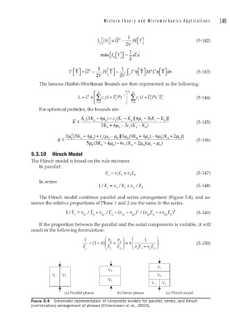
5.3.10 Hirsch Model
The Hirsch model is based on the rule mixtures.
In parallel:
E = v E + v E (5-147)
c 11 2 2
In series:
1/E = v /E + v /E (5-148)
c 1 1 2 2
The Hirsch model combines parallel and series arrangement (Figure 5.4), and as-
sumes the relative proportions of Phase 1 and 2 are the same in the series.
1/E = v /E + v /E + (v + v ) /(v E + + v E ) ) 2 (5-149)
2
c 1s 1 2s 2 1p 2p 1p 2 2p 2
If the proportion between the parallel and the serial components is variable, it will
result in the following formulation:
1 ⎛ v 1 v ⎞ ⎛ 1 ⎞
−
2
= ( 1 x) ⎜ + ⎟ + x ⎜ ⎟ (5-150)
E ⎝ E E 2 ⎠ ⎝ vE + v E 2 ⎠
c 1 1 1 2
V 1
V 1
V 1 V 2 V 2
V 2
V 1 V 2
(a) Parallel phases (b) Series phases (c) Hirsch model
FIGURE 5.4 Schematic representation of composite models for parallel, series, and Hirsch
(combination) arrangement of phases (Christensen et al., 2003).