Page 193 - Mechanics of Asphalt Microstructure and Micromechanics

Fundamentals of Phenomenological Models 185

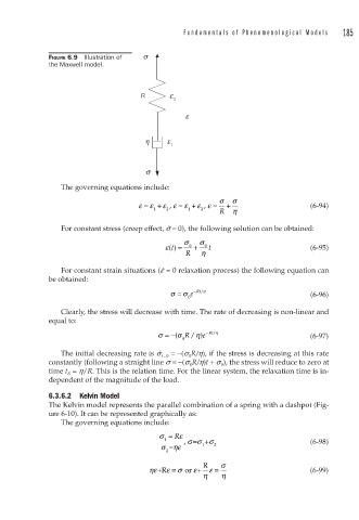
FIGURE 6.9 Illustration of σ
the Maxwell model.

R ε
2
ε

η ε
1

σ

The governing equations include:
σ σ
ε = ε + ε ε = ε + ε ε = + (6-94)
,
,
1 2 1 2 R η

For constant stress (creep effect, s˙ = 0), the following solution can be obtained:
σ σ
ε() = 0 + 0 t (6-95)
t
R η

For constant strain situations (e˙ = 0 relaxation process) the following equation can
be obtained:
σ = σ e −Rt/ η (6-96)
0
Clearly, the stress will decrease with time. The rate of decreasing is non-linear and
equal to:

σ
σ =−( R / η)e −Rt / η (6-97)
0
˙
The initial decreasing rate is s t=0 = −(s 0 R/h), if the stress is decreasing at this rate
constantly (following a straight line s = −(s 0 R/h)t + s 0 ), the stress will reduce to zero at
time t R = h/R. This is the relation time. For the linear system, the relaxation time is in-
dependent of the magnitude of the load.

6.3.6.2 Kelvin Model
The Kelvin model represents the parallel combination of a spring with a dashpot (Fig-
ure 6-10). It can be represented graphically as:
The governing equations include:
σ = R ε
1 ,= σ (6-98)
σσ +
σ = ηε 1 2
2
ηε+R = σ or ε+ R ε = σ (6-99)
ε
η η