Page 192 - Mechanics of Asphalt Microstructure and Micromechanics

184 Ch a p t e r S i x

ε t ()
If the creep compliance is Ct() = , the strain response (measured at time t) due
σ
0
to the load increment Δs at time instant t should be Δε = ΔσCt( − τ H t − τ) .
(
)
Where H(t − t) is the step function.
H(t − t) = 0 for t t (6-90)
1 for t t
Decompose the complex loading into a series of incremental loading, and the over-
all response can be represented as:
N
N
ε( ) ≈ ∑ Δ ε( ) ≈ ∑ Δ σ (t − τ ) (t − τ ) (6-91)
C
H
t
i
i
i
i
i=1 i=1
When Δσ → 0 , the above summation can be represented as an integral.
i
ε( ) = ∫ t d σ (Ct − τ) (t − τ) = ∫ t ( Ct − τ) (t − τ σ (6-92)
H
H
)
d
t
0 0
Since t t, the above integral can be simplified as ε()t = ∫ 0 t ( C t − τ σ .
d
)
ε() [ (t − τ στ)]| + t στ)dC − τ) (6-93)
=
t
(
(
t
(t
C
)
0 ∫ 0
6.3.6 Simple Linear Models
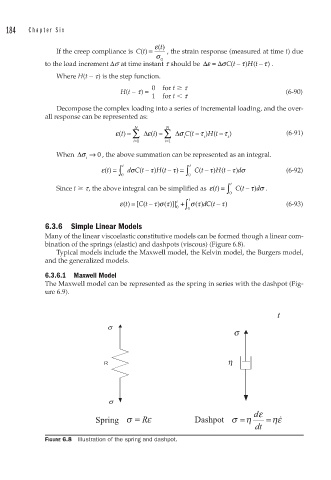
Many of the linear viscoelastic constitutive models can be formed though a linear com-
bination of the springs (elastic) and dashpots (viscous) (Figure 6.8).
Typical models include the Maxwell model, the Kelvin model, the Burgers model,
and the generalized models.
6.3.6.1 Maxwell Model
The Maxwell model can be represented as the spring in series with the dashpot (Fig-
ure 6.9).
t
σ
σ
η
R

σ
dε
Spring σ = Rε Dashpot σ = η = ηε
dt

FIGURE 6.8 Illustration of the spring and dashpot.