Page 130 - Mechatronic Systems Modelling and Simulation with HDLs

6.3 CONTINUUM MECHANICS 119

from the collection of finite elements in symbolic form, and then to directly formu-
late this in a hardware description language. In theory this is correct. However, the
handling of the equations causes massive problems. This is firstly the case if we
want to parameterise the elements geometrically and not on the basis of the entries
in the element matrix. The same applies in the nonlinear consideration if the mass
and stiffness matrices of the finite elements are dependent upon the current state
of deformation and have to be drawn up afresh depending upon deflection. In both
cases the complete rule for the creation of the element matrices must be included
in the equation system, as must the conversion from the element matrices into the
system matrix. This allows the volume of equations to explode and the resulting
equation system is thus beyond any meaningful calculation.
It therefore makes sense to initially consider the finite elements individually and
to build the rule for the creation of the element matrices into the model in ques-
tion. This could, for example, be achieved by embedding a C routine, capable of
generating suitable element matrices as required, into the model. This corresponds
with the numerical simulation of multibody systems. The question is also raised
of how to move from element behaviour to system behaviour. Ideally, the system
behaviour would be found by composing the finite elements in a circuit simulator.
This first requires a link between electronic quantities and mechanical degrees of
freedom. Here mechanical deflections are represented by electrical potentials and
mechanical forces and moments by electrical currents. The linking of two finite
2
elements effects a scleronomic constraint between the element degrees of freedom
in question, and thus the amalgamation of the degrees of freedom in question to a
single system degree of freedom. This is the expected behaviour for voltages and
positions. Furthermore, the currents are added at these points, as is also expected
of forces and moments.

The generation of element matrices
In what follows the example of the shear-resistant beam element will be used to
demonstrate how such a finite element can be formulated in hardware description
languages. To achieve this two main problems have to be solved. Firstly the mass
and stiffness matrices in question have to be generated. Secondly the element
matrices have to be transformed into the system matrices, which represents the
behaviour of the entire structure.
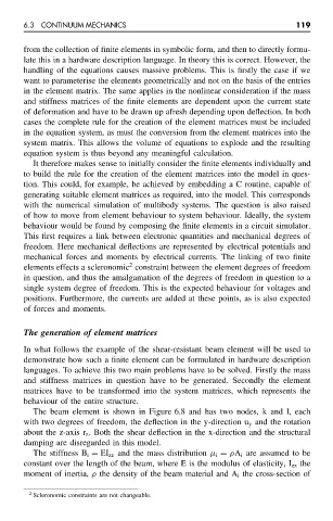
The beam element is shown in Figure 6.8 and has two nodes, k and l, each
with two degrees of freedom, the deflection in the y-direction u y and the rotation
about the z-axis r z . Both the shear deflection in the x-direction and the structural
damping are disregarded in this model.
The stiffness B i = EI zz and the mass distribution µ i = ρA i are assumed to be
constant over the length of the beam, where E is the modulus of elasticity, I zz the
moment of inertia, ρ the density of the beam material and A i the cross-section of

2 Scleronomic constraints are not changeable.