Page 132 - Mechatronic Systems Modelling and Simulation with HDLs

6.3 CONTINUUM MECHANICS 121

Now, if the behaviour of a mechanical continuum is to be reconstructed in a
circuit simulator it is reasonable to keep the modelling close to the actual deter-
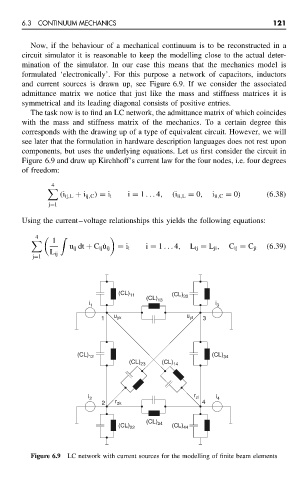
mination of the simulator. In our case this means that the mechanics model is
formulated ‘electronically’. For this purpose a network of capacitors, inductors
and current sources is drawn up, see Figure 6.9. If we consider the associated
admittance matrix we notice that just like the mass and stiffness matrices it is
symmetrical and its leading diagonal consists of positive entries.
The task now is to find an LC network, the admittance matrix of which coincides
with the mass and stiffness matrix of the mechanics. To a certain degree this
corresponds with the drawing up of a type of equivalent circuit. However, we will
see later that the formulation in hardware description languages does not rest upon
components, but uses the underlying equations. Let us first consider the circuit in
Figure 6.9 and draw up Kirchhoff’s current law for the four nodes, i.e. four degrees
of freedom:
4

(i ij,L + i ij,C ) = i i i = 1 ... 4, (i ii,L = 0, i ii,C = 0) (6.38)
j=1
Using the current–voltage relationships this yields the following equations:

1
4

u ij dt + C ij ˙u ij = i i i = 1 ... 4, L ij = L ji , C ij = C ji (6.39)
L ij
j=1

(CL) 11 (CL)
(CL) 13 33
i 1 i 3
1 u yk u yl 3

(CL) 12 (CL) 34
(CL) 23 (CL) 14

i 2 r zl i 4
2 r zk 4

(CL)
(CL) 22 24 (CL) 44

Figure 6.9 LC network with current sources for the modelling of finite beam elements