Page 134 - Mechatronic Systems Modelling and Simulation with HDLs

6.3 CONTINUUM MECHANICS 123

This equation system has the same structure as the LC network, see equation (6.43).
We now have to identify the individual components of the two matrix equations
with each other, i.e.:

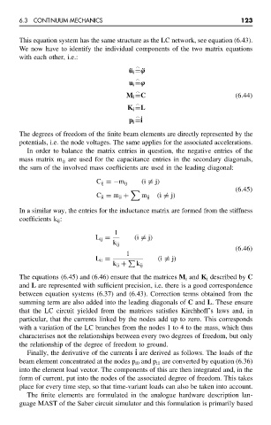
¨ u i = ¨ϕ

u i =ϕ

M i =C (6.44)

K i =L

p i =i ˙

The degrees of freedom of the finite beam elements are directly represented by the
potentials, i.e. the node voltages. The same applies for the associated accelerations.
In order to balance the matrix entries in question, the negative entries of the
mass matrix m ij are used for the capacitance entries in the secondary diagonals,
the sum of the involved mass coefficients are used in the leading diagonal:

C ij =−m ij (i = j)
(6.45)

C ii = m ii + m ij (i = j)
In a similar way, the entries for the inductance matrix are formed from the stiffness
coefficients k ij :
1
L ij = (i = j)
k ij
(6.46)
1
L ii = (i = j)
k ii + k ij
The equations (6.45) and (6.46) ensure that the matrices M i and K i described by C
and L are represented with sufficient precision, i.e. there is a good correspondence
between equation systems (6.37) and (6.43). Correction terms obtained from the
summing term are also added into the leading diagonals of C and L. These ensure
that the LC circuit yielded from the matrices satisfies Kirchhoff’s laws and, in
particular, that the currents linked by the nodes add up to zero. This corresponds
with a variation of the LC branches from the nodes 1 to 4 to the mass, which thus
characterises not the relationships between every two degrees of freedom, but only
the relationship of the degree of freedom to ground.
˙
Finally, the derivative of the currents i are derived as follows. The loads of the
beam element concentrated at the nodes p i0 and p i1 are converted by equation (6.36)
into the element load vector. The components of this are then integrated and, in the
form of current, put into the nodes of the associated degree of freedom. This takes
place for every time step, so that time-variant loads can also be taken into account.
The finite elements are formulated in the analogue hardware description lan-
guage MAST of the Saber circuit simulator and this formulation is primarily based