Page 137 - Mechatronic Systems Modelling and Simulation with HDLs

126 6 MECHANICS IN HARDWARE DESCRIPTION LANGUAGES

and to represent this using, for example, the method of finite differences on a
system of ordinary differential equations, which again can be directly formulated
in a hardware description language. The second method relies upon analytical
solutions of the partial differential equations in question which are, however, rarely
known. Finally, the last two options — the Ritz and Galerkin approaches — attempt
to describe bending structures on the basis of a calculus of variations.

Partial differential equations and finite differences

A classical approach to the consideration of the physics of bending structures is to
derive a partial differential equation, which can, for example, be represented as a
set of ordinary differential equations by the method of finite differences. This step
is necessary because analogue hardware description languages cannot in general
process partial differential equations directly. The process described was first used
by Lee and Wise [224] in order to investigate pressure sensor systems in bulk
micromechanics, in which the (quasi-static) solution was built into the respective
circuit simulator. In [322], [323] and [324] Pelz et al. transferred this solution
from the tool level to the model level, where the automatic translation of partial
differential equations (in one dimension) into hardware description languages and
equivalent Spice net lists was investigated in particular. Consideration was also
given to mechanical kinetics. Mrˇ carica et al. [278] also use this approach to con-
sider two-dimensional, partial differential equations, favouring a direct formulation
in the in-house hardware description language AleC++. Finally, Klein and Gerlach
[195] break up a bending plate into fragments in their approach, and models in an
analogue hardware description language are then applied to each of these. These
can again be connected to a circuit simulation, thus facilitating the co-simulation
of continuum mechanics and electronics. The formulation leads to a system model
that is mathematically equivalent to the method of finite differences.
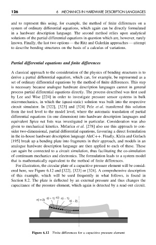
For illustration, the circular plate of a capacitive pressure element will be consid-
ered here, see Figure 6.12 and [322], [323] or [324]. A comprehensive description
of this example, which will be used frequently in what follows, is found in
Section 8.2. The plate is deflected by an external pressure and thus changes the
capacitance of the pressure element, which again is detected by a read-out circuit.

r(i + 1) r(i) r(i − 1)
r(i + 2)
r(i − 2)

Figure 6.12 Finite differences for a capacitive pressure element