Page 136 - Mechatronic Systems Modelling and Simulation with HDLs

6.3 CONTINUUM MECHANICS 125

y y y
F y (t) F y (t)

x x
l
l/2
(a) (b)

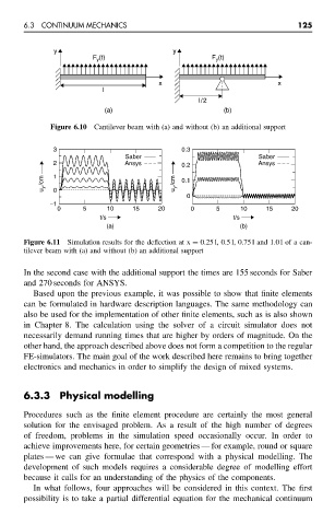
Figure 6.10 Cantilever beam with (a) and without (b) an additional support

3 0.3
Saber Saber
2 Ansys 0.2 Ansys

u y /cm 1 u y /cm 0.1
0
0
−1
0 5 10 15 20 0 5 10 15 20
t/s t/s
(a) (b)
Figure 6.11 Simulation results for the deflection at x = 0.25 l, 0.5 l, 0.75 l and 1.0 l of a can-
tilever beam with (a) and without (b) an additional support

In the second case with the additional support the times are 155 seconds for Saber
and 270 seconds for ANSYS.
Based upon the previous example, it was possible to show that finite elements
can be formulated in hardware description languages. The same methodology can
also be used for the implementation of other finite elements, such as is also shown
in Chapter 8. The calculation using the solver of a circuit simulator does not
necessarily demand running times that are higher by orders of magnitude. On the
other hand, the approach described above does not form a competition to the regular
FE-simulators. The main goal of the work described here remains to bring together
electronics and mechanics in order to simplify the design of mixed systems.

6.3.3 Physical modelling

Procedures such as the finite element procedure are certainly the most general
solution for the envisaged problem. As a result of the high number of degrees
of freedom, problems in the simulation speed occasionally occur. In order to
achieve improvements here, for certain geometries — for example, round or square
plates — we can give formulae that correspond with a physical modelling. The
development of such models requires a considerable degree of modelling effort
because it calls for an understanding of the physics of the components.
In what follows, four approaches will be considered in this context. The first
possibility is to take a partial differential equation for the mechanical continuum