Page 242 - Mechatronics for Safety, Security and Dependability in a New Era

Ch46-I044963.fm Page 226 Tuesday, August 1, 2006 3:57 PM
Ch46-I044963.fm
226
226 Page 226 Tuesday, August 1, 2006 3:57 PM
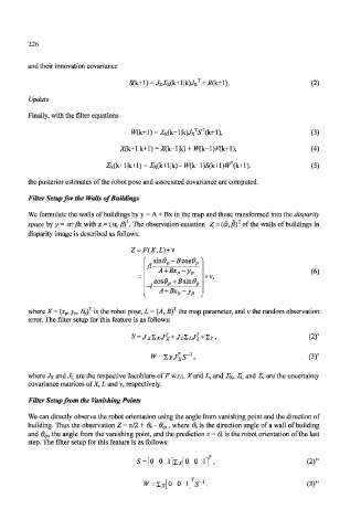
and their innovation covariance

T
S(k+]) = J xE x(k+\ |k>/x + #(k+l). (2)
Update

Finally, with the filter equations

IV(k+l) = J7 x (k+l|k)./xV(k+l), (3)
Jf(k+l|k+l) = Jf(k+l|k) + W(k+\)V(k+\\ (4)

1
2k(k+l|k+l) = 2x(k+l|k) - W{k+l)S(\<.+\)W {k+\). (5)
the posterior estimates of the robot pose and associated covariance are computed.

Filter Setup for the Walls of Buildings

We formulate the walls of buildings by y = A + Bx in the map and those transformed into the disparity
T
space by y = a+fix with z = (a, J3) . The observation equation Z = (a,J3) J of the walls of buildings in
disparity image is described as follows:
' = F(X,L) + v

fl Sm0p ~
A + Bx p-y p (6)
+ v,
-I
A + Bx p-y p

T
where X= (x p, y p, 9 P) is the robot pose, L = (A, B) T the map parameter, and v the random observation
error. The filter setup for this feature is as follows:
I.v, (2)'

(3)'

where Jx and JL are the respective Jacobians of F w.r.t. Xand L, and Ex, EL and E, are the uncertainty
covariance matrices of X, L and v, respectively.
Filter Setup from the Vanishing Points

We can directly observe the robot orientation using the angle from vanishing point and the direction of
building. Thus the observation Z = n/2 + Ob- 0 vp , where Of, is the direction angle of a wall of building
and 0,-p, the angle from the vanishing point, and the prediction z = 0 r is the robot orientation of the last
step. The filter setup for this feature is as follows:

[
= 0 0 l]x A{0 0 I]'', (2)"
(3)"