Page 243 - Mechatronics for Safety, Security and Dependability in a New Era

Ch46-I044963.fm Page 227 Tuesday, August 1, 2006 3:57 PM
Tuesday, August
3:57 PM
1, 2006
Page 227
Ch46-I044963.fm
227
227
Filter Setup for the Corners of Buildings
After we found the corresponding corner of building to the boundary line Z = (x, d) T in the disparity
space, the observation equation can be described like the following equation:
= H(X,M) + v
m
' ( x -x p)s'm0 p -(m y -y p)cos0 p
(m x-x p)cos0 p+(m y-y p)sm0 p (7)
+ v,
fl
-
(m x x p ) cos 6 p + (m y -y p)sin0 p
where M = (m x, m v) T is the coordinates of the building corner on the map. The filter setup for this
feature is as follows:
T T (2)'"
S = Jx^xJ x + JMT.MJ M
M
(3)'"

EXPERIMENTAL RESULTS
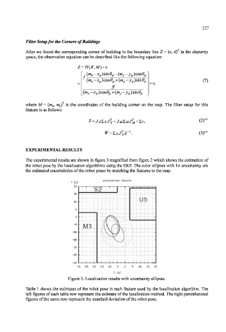
The experimental results are shown in figure 3 magnified from figure 2 which shows the estimation of
the robot pose by the localization algorithms using the EKF. The color ellipses with 1 cr uncertainty are
the estimated uncertainties of the robot poses by matching the features to the map.

Localization Results
T [m]
20
B2 1
15
10
5
0
-5
:M3
-10
-15
-20
-25

-30 -25 -20 -15 -10 -5 10 15 20
X [m]
Figure 3: Localization results with uncertainty ellipses.

Table 1 shows the estimates of the robot pose in each feature used by the localization algorithm. The
left figures of each table row represent the estimate of the localization method. The right parenthesized
figures of the same row represent the standard deviation of the robot pose.