Page 123 - MODELING OF ASPHALT CONCRETE

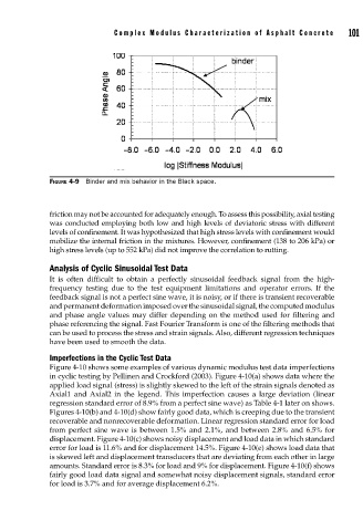
Complex Modulus Characterization of Asphalt Concr ete 101

FIGURE 4-9 Binder and mix behavior in the Black space.

friction may not be accounted for adequately enough. To assess this possibility, axial testing
was conducted employing both low and high levels of deviatoric stress with different
levels of confinement. It was hypothesized that high stress levels with confinement would
mobilize the internal friction in the mixtures. However, confinement (138 to 206 kPa) or
high stress levels (up to 552 kPa) did not improve the correlation to rutting.

Analysis of Cyclic Sinusoidal Test Data
It is often difficult to obtain a perfectly sinusoidal feedback signal from the high-
frequency testing due to the test equipment limitations and operator errors. If the
feedback signal is not a perfect sine wave, it is noisy, or if there is transient recoverable
and permanent deformation imposed over the sinusoidal signal, the computed modulus
and phase angle values may differ depending on the method used for filtering and
phase referencing the signal. Fast Fourier Transform is one of the filtering methods that
can be used to process the stress and strain signals. Also, different regression techniques
have been used to smooth the data.

Imperfections in the Cyclic Test Data
Figure 4-10 shows some examples of various dynamic modulus test data imperfections
in cyclic testing by Pellinen and Crockford (2003). Figure 4-10(a) shows data where the
applied load signal (stress) is slightly skewed to the left of the strain signals denoted as
Axial1 and Axial2 in the legend. This imperfection causes a large deviation (linear
regression standard error of 8.9% from a perfect sine wave) as Table 4-1 later on shows.
Figures 4-10(b) and 4-10(d) show fairly good data, which is creeping due to the transient
recoverable and nonrecoverable deformation. Linear regression standard error for load
from perfect sine wave is between 1.5% and 2.1%, and between 2.8% and 6.5% for
displacement. Figure 4-10(c) shows noisy displacement and load data in which standard
error for load is 11.6% and for displacement 14.5%. Figure 4-10(e) shows load data that
is skewed left and displacement transducers that are deviating from each other in large
amounts. Standard error is 8.3% for load and 9% for displacement. Figure 4-10(f) shows
fairly good load data signal and somewhat noisy displacement signals, standard error
for load is 3.7% and for average displacement 6.2%.