Page 125 - MODELING OF ASPHALT CONCRETE

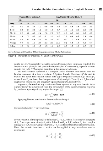
Complex Modulus Characterization of Asphalt Concr ete 103

Standard Error for Load, % Avg. Standard Error for Displ., %
Hz Hz
Temp. 25 10 5 1 0.5 0.1 25 10 5 1 0.5 0.1
−9°C 8.9 6.0 3.4 1.2 0.8 0.6 9.6 14.4 5.8 3.8 10.4 3.3
4.4°C 8.6 3.7 2.3 1.2 1.0 1.5 8.7 4.9 4.0 3.1 3.0 2.8
21.1°C 9.5 5.6 3.6 2.4 2.0 2.2 12.0 9.5 3.9 3.1 6.9 6.5
37.8°C 11.6 7.3 5.5 3.2 3.1 2.1 14.5 7.6 6.4 6.8 7.4 8.4
54.4°C 8.3 9.1 6.8 5.3 4.4 3.7 10.0 9.0 7.2 6.8 6.1 6.2
Average 9.4 6.3 4.3 2.7 2.3 2.0 11.0 9.1 5.5 4.7 6.8 5.4
St.Dev. 1.3 2.0 1.8 1.7 1.5 1.1 2.3 3.5 1.5 1.9 2.7 2.3

Source: Pellinen and Crockford 2003, with permission from RILEM Publications.
TABLE 4-1 Standard Error of Estimate for Deviation of Sine Wave

points (m > 2). To completely describe a given frequency, two values are required: the
magnitude and phase, or real part and imaginary part. Consequently, N points in time-
domain can yield N/2 complex quantities in the frequency domain.
The linear Fourier spectrum is a complex valued function that results from the
Fourier transform of a time waveform. A System Transfer Function H(f) is used to
transfer the input data x(t) and output data y(t) to frequency domain S (f) and S (f),
x y
where S and S are linear Fourier spectrums of x(t) and y(t). Thus, S and S have real
x y x y
(in phase or coincident) and imaginary (quadrature) parts, respectively.
In general, the result of any continuous linear system on any time domain input
signal x(t) may be determined from the convolution of the system impulse response
h(t), with the input signal x(t), to give the output y(t).

∞
τ
yt() = ∫ −∞ h( )( −τ τ (4-10)
d )
t
Applying Fourier transform to the convolution integral
Sf () = S f H f ()
()
y x (4-11)
the transfer function H can be defined
OUTPUT S
H = = y (4-12)
INPUT S x
∗
∗
Power spectrum of the input x(t) is defined as G = S S , where S is complex conjugate
xx x x x
∗
∗
of S . Power spectrum of output y(t) is defined as G = S S , where S is a complex
x yy y y y
∗
conjugate of S . Gross power spectrum is G = S S and it contains the phase information.
y yx y x
Then, the transfer function H, which can be applied to any waveform, can be
defined as:
S S * G
H = y ⋅ x = yx (4-13)
S x S * x G xx