Page 181 - Modeling of Chemical Kinetics and Reactor Design

Reaction Rate Expression 151

All other reversible second-order rate equations have the same
solution with the boundary conditions assumed in Equation 3-176.
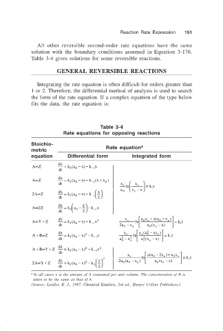
Table 3-4 gives solutions for some reversible reactions.

GENERAL REVERSIBLE REACTIONS

Integrating the rate equation is often difficult for orders greater than
1 or 2. Therefore, the differential method of analysis is used to search
the form of the rate equation. If a complex equation of the type below
fits the data, the rate equation is:

Table 3-4
Rate equations for opposing reactions

Stoichio-
Rate equation a
metric
equation Differential form Integrated form
x −
[
AZ dx = ka − ) k x 
(
−1
1
0
dt
 
x −
+
[
(
AZ dx = ka − ) k ( x x ) 
0
−1
1
0
dt   x e ln   x e   = kt
1
x
x 
e
x −
[
2 AZ dx = ka − ) k −1      a 0  x − 
(
1
0
dt 2 

dx  x  
A[2 Z = ka −  − kx

1
0
−1
dt 2  
x a −
[ +
x −
e
0 e
AY Z dx = ka − ) k x 2 x e ln   ax + ( 0 x )   = kt
(
0
−1
1
1
(
dt 2 2a − x e  ax − x) 
e
0
0
2
(
0
+ [
e
e
AB Z dx = ka − x) 2 − k x x e ln   xa − xx )   = kt
(
−
1
1
0
1
2
2
dt a − x 2  ax − x) 
(
0 e 0 e
+ [
+
2
)
(
AB Y Z dx = ka − x) − kx 2 
−
0
1
1
dt   x e ln   xa ( 0 − 2 x ) + a x   = kt
0
e
e
x
[
+
0
e
0
2
2AY Z dx = ka 0 − x ) − k 1   2   2 aa ( 0 − x )  ax ( e − x)  1
(
1
dt  2   
a
In all cases x is the amount of A consumed per unit volume. The concentration of B is
taken to be the same as that of A.
(Source: Laidler, K. J., 1987. Chemical Kinetics, 3rd ed., Harper Collins Publishers.)