Page 516 - Modelling in Transport Phenomena A Conceptual Approach

496 APPENDIX A. MATHEMATICAL PRBLIMZVARLES

3. Fitting short sections of the data by arbitrary functions.
4. Using the difference table method, i.e., plotting the differences and smoothing
the differences graphically.
De Nevers also points out the fact that although the value of dyldx obtained
by any of the above four methods is approximately equal, the value of &y/dx2 is
extremely sensitive to the method used.
In the case of the graphical method, there are infinite number of ways of drawing
the curve through the data points. As a result, the slope of the tangent will be
affected by the mechanics of drawing the curved line and the tangent.
The availability of computer programs makes the second and the third methods
highly attractive. However, since the choice of the functional form of the equation
is highly arbitrary, the final result is almost as subjective and biased as the use of
a Fkench curve.
Two methods, namely, DouglassAvakian (1933) and Whitaker-Pigford (1960)
methods, are worth mentioning among the third approach. Both of these methods
require the values of the independent variable, x, be equally spaced by an amount
Ax.

A. 5.1 Douglass-Avakian Met hod
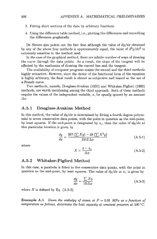
In this method, the value of dyldx is determined by fitting a fourth-degree polyn+
mial to seven consecutive data points, with the point in question as the mid-point,
by least squares. If the mid-point is designated by x,, then the value of dyldx at
this particular location is given by

(A.5-1)

where
x - xc
X=- (A.52)
Ax
A.5.2 Whitaker-Pigford Met hod

In this case, a parabola is fitted to five consecutive data points, with the point in
question as the mid-point, by least squares. The value of dylh at xc is given by

(A.53)

where X is defined by Eq. (AS-2).

Example A.l Given the enthalpy of steam at P = 0.01 MPa as a function of
temperature as follows, determine the heat capacity at constant p~~.~sum 500 "C.
at