Page 518 - Modelling in Transport Phenomena A Conceptual Approach

498 APPENDIX A. MATHEMATICAL PRELIMINARTES

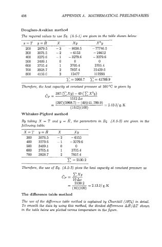
Douglass- Avakian method
The required values to use Eq. (A.5-1) are given in the table shown below:
x=T X x3u
200 2879.5 -3 - 8638.5 - 77746.5
300 3076.5 -2 - 6153 - 24612
400 3279.6 -1 - 3279.6 - 3279.6
500 3489.1 0 0 0
600 3705.4 1 3705.4 3705.4
700 3928.7 2 7857.4 31429.6
800 4159.0 3 12477 112293
= 5968.7 = 41789.9
Therefore, the heat capacity at constant pressure at 5OOOC is given by

397 (E Xy) - 49 ( x3y)
A
cp =
1512 Ax
- (397)(5968.7) - (49)(41,789.9)
-
( 15 12) (1 00) = 2.13 J/ g. K
Whitaker-Pigford method
By taking X = T and y = H, the parameters in Eq. (A.5-3) are given in the
following table:
X=T y=H X XY
300 3076.5 -2 - 6153
400 3279.6 -1 -3279.6
500 3489.1 0 0
600 3705.4 1 3705.4
700 3928.7 2 7857.4
E = 2130.2
Therefore, the we of Eq. (A.5-3) gives the heat capacity at constant pressure as

EXY
cp = -
A
10 Ax

The difference table method
The use of the diflerence table method is explained by Churchill (197.) in detail.
To smooth the data by using this method, the divided dzfferences AH/AT shown
in the table below are plotted versus temperature in the figure.