Page 520 - Modelling in Transport Phenomena A Conceptual Approach

500 APPENDIX A. MATHEMATICAL PRELIMINARlEs

Each line represents the average value of dH/dT over the specified temperature
range. The smooth curve should be drawn so as to equalize the area under the
group of bars. From the figure, the heat capacity at constant pressure at 500°C is
2.15 J/ g. K.

A.6 REGRJESSION AND CORBICLATION

To predict the mechanism of a process, we often need to know the relationship of
one process variable to another, i.e., how the reactor yield depends on pressure. A
relationship between the two variables x and y, measured over a range of values, can
be obtained by proposing linear relationships first, because they are the simplest.
The analyses we use for this are correlation, which indicates whether there is indeed
a linear relationship, and regression, which finds the equation of a straight line that
best fits the observed x - y data.

A.6.1 Simple Linear Regression

The equation describing a straight line is
y=ax+b (A.6-1)
where a denotes the slope of the line and b denotes the y-axis intercept. Most
of the time the variables x and y do not have a linear relationship. However,
transformation of the variables may result in a linear relationship. Some examples
of transformation are given in Table A.2. Thus, linear regression can be applied
even to nonlinear data.

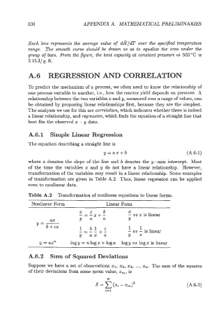
Table A.2 Transformation of nonlinear equations to linear forms.
Nonlinear Form Linear Form
x c b X
- ws x is linear
ax ;=a"+; Y
y=-
1
1
1
bl c
b+cx -=-- +- - ws - is linear
y ax a Y =
y = ax" logy=nlogx+loga logyvs logxislinear
A.6.2 Sum of Squared Deviations

Suppose we have a set of observations 21, x2, 33, ..., xn. The sum of the squares
of their deviations from some mean value, x,, is
N
(A.6-2)