Page 523 - Modelling in Transport Phenomena A Conceptual Approach

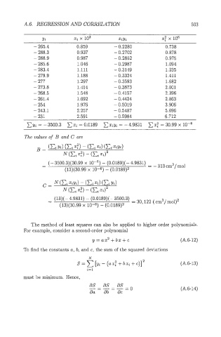
A.6. REGRESSION AND CORRELATION 503

Yi xi x 103 XiYi x: x 106
- 265.4 0.859 - 0.2280 0.738
- 288.3 0.937 - 0.2702 0.878
- 288.9 0.987 - 0.2852 0.975
- 285.6 1.046 - 0.2987 1.094
- 283.4 1.111 - 0.3149 1.235
- 279.9 1.188 - 0.3324 1.41 1
- 277 1.297 - 0.3593 1.682
- 273.8 1.414 - 0.3873 2.001
- 268.5 1.548 - 0.4157 2.396
- 261.4 1.692 - 0.4424 2.863
- 254 1.976 - 0.5019 3.906
- 243.1 2.257 - 0.5487 5.096
- 231 2.591 - 0.5984 6.712
yi = - 3500.3 xi = 0.0189 ~iyj = - 4.9831 X: = 30.99 x

The values of B and C are

- (- 3500.3)(30.99 x - (0.0189)(- 4.9831) = - 313 cm3/ mol
-
(13)(30.99 x - (0.0189)2

The method of least squares can also be applied to higher order polynomials.
For example, consider a second-order polynomial
y = a x2 + b x + c (A.6-12)

To find the constants a, b, and c, the sum of the squared deviations
N
s = [yi - (UX? + bXi + c)] 2 (A.6-13)
i=I
must be minimum. Hence,
(A.6-14)