Page 567 - Modelling in Transport Phenomena A Conceptual Approach

B.2. SECONDORDER LINEAR DIFFERENTTAL EQUATIONS 547

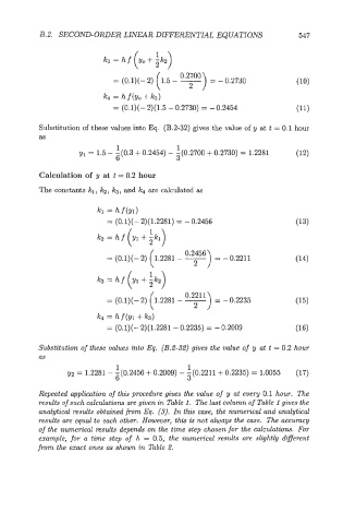
k3 = hf (Yo + ik2)

k4 = h f (yo + k3)
= (O.l)(- 2)(1.5 - 0.2730) = - 0.2454 (11)

Substitution of these values into Ea. (B.2-32) gives the value of y at t = 0.1 hour
as
1 1
~1 = 1.5 - -(0.3 + 0.2454) - -(0.2700 + 0.2730) = 1.2281
6 3

CalcuIation of y at t = 0.2 hour
The constants kl, k2, k3, and k4 are calculated as

kl = hf (Yl)
= (O.l)(- 2)(1.2281) = - 0.2456

2

2
k4 = h f (Y1+ k3)
= (O.l)(- 2)( 1.2281 - 0.2235) = - 0.2009

Substitution of these values into Eq. (B.2-32) gives the value of y at t = 0.2 hour
as
1 1
~2 = 1.2281 - -(0.2456 + 0.2009) - -(0.2211+ 0.2235) = 1.0055 (17)
6 3

Repeated application of this procedure gives the value of y at evesy 0.1 hour. The
results of such calculations are given in Table 1. The last column of Table 1 gives the
analytical results obtained from Eq. (3). In this case, the numerical and analytical
results are equal to each other. However, this is not always the case. The accuracy
of the numerical results depends on the time step chosen for the calculations. For
example, for a time step of h = 0.5, the numerical results are slightly diflerent
from the exact ones as shown in Table 2.