Page 572 - Modelling in Transport Phenomena A Conceptual Approach

552 APPENDIX 33. SOLUTIONS OF DFFEmNT1A.L EQUATIONS

Substitution of kl --t k4 and C1 --t 4 into Eqs. (B.2-39) and (B.S4O), respectively,
gives the values of y1 and z1 as
1 1
91 = 1 - - (0.0200 + 0.0196) - -(0.0198 + 0.0198) = 0.9802 (26)
6 3
1 1
z1 = 0 + - (0 + 6.8086 x + -(3.5 x + 3.4032 x
6 3
= 3.4358 x (27)
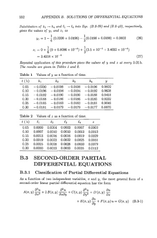
Repeated application of this procedure gives the values of y and z at every 0.05 h.
The results are given in Tables 1 and 2.

Thble 1 Values of y as a function of time.
t (h) kl IC2 k3 k4 Y
0.05 - 0.0200 - 0.0198 - 0.0198 - 0.0196 0.9802
0.10 - 0.0196 - 0.0194 - 0.0194 - 0.0192 0.9608
0.15 - 0.0192 - 0.0190 - 0.0190 - 0.0188 0.9418
0.20 - 0.0188 - 0.0186 - 0.0186 - 0.0185 0.9232
0.25 - 0.0185 - 0.0183 - 0.0183 - 0.0181 0.9049
0.30 - 0.0181 - 0.0179 - 0.0179 - 0.0177 0.8870

nble 2 Values of z as a function of time.

0.05 0.0000 0.0004 0.0003 0.0007 0.0003
0.10 0.0007 0.0010 0.0010 0.0013 0.0013
0.15 0.0013 0.0016 0.0016 0.0019 0.0029
0.20 0.0019 0.0022 0.0022 0.0025 0.0051
0.25 0.0025 0.0028 0.0028 0.0030 0.0079
0.30 0.0030 0.0033 0.0033 0.0035 0.0112

B.3 SECOND-ORDER PARTIAL
DIFFEFtENTIAL EQUATIONS

B.3.1 Classification of Partial Differential Equations

As a function of two independent variables, x and y, the most general form of a
second-order linear partial differential equation has the form

azl
+ E(z, 9) - + F(x,Y) u = G(z, 9) (B.3-1)
aY