Page 568 - Modelling in Transport Phenomena A Conceptual Approach

548 APPENDIX B. SOLUTIONS OF DLEFERENTIAL EQUATIONS

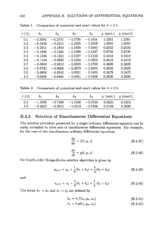
Table 1 Comparison of numerical and exact values for h = 0.1.

t (h) kl IE2 k3 k4 Y (num.) Y (exact)
0.1 - 0.3000 - 0.2700 - 0.2730 - 0.2454 1.2281 1.2281
0.2 - 0.2456 - 0.2211 - 0.2235 - 0.2009 1.0055 1.0055
0.3 - 0.2011 - 0.1810 - 0.1830 - 0.1645 0.8232 0.8232
0.4 - 0.1646 - 0.1482 - 0.1498 - 0.1347 0.6740 0.6740
0.5 - 0.1348 - 0.1213 - 0.1227 - 0.1103 0.5518 0.5518
0.6 - 0.1104 - 0.0993 - 0.1004 - 0.0903 0.4518 0.4518
0.7 - 0.0904 - 0.0813 - 0.0822 - 0.0739 0.3699 0.3699
0.8 - 0.0740 - 0.0666 - 0.0673 - 0.0605 0.3028 0.3028
0.9 - 0.0606 - 0.0545 - 0.0551 - 0.0495 0.2479 0.2479
1.0 - 0.0496 - 0.0446 - 0.0451 - 0.0406 0.2030 0.2030

Table 2 Comparison of numerical and exact values for h = 0.5.

t (h) kl k2 k3 IC4 y (num.) y (exact)
0.5 - 1.5000 -0.7500 - 1.1250 -0.3750 0.5625 0.5518
1.0 - 0.5625 -0.2813 -0.4219 -0.1406 0.2109 0.2030

B.2.5 Solution of Simultaneous Differential Equations
The solution procedure presented for a single ordinary differential equation can be
easily extended to solve sets of simultaneous differential equations. For example,
for the case of two simultaneous ordinary differential equations

(B.2-37)

da
- = g(t, Y, 4 (B.2-38)
dt
the fourth-order Runge-Kutta solution algorithm is given by

(B.239)

and
1 1
3
Zn+l = 4a + $1 + t4) + - (e2 + e3) (B .2-40)
The terms ki + k4 and el + t4 are defined by
(B.2-41)
(B.2-42)