Page 150 - Modern Analytical Chemistry

1400-CH05 9/8/99 3:59 PM Page 133

Chapter 5 Calibrations, Standardizations, and Blank Corrections 133

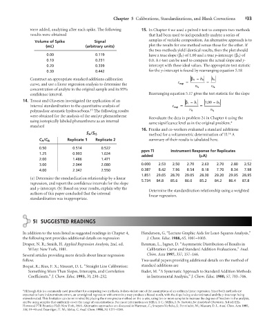
were added, analyzing after each spike. The following 15. In Chapter 4 we used a paired t-test to compare two methods
results were obtained that had been used to independently analyze a series of
Volume of Spike Signal samples of variable composition. An alternative approach is to
(mL) (arbitrary units) plot the results for one method versus those for the other. If
the two methods yield identical results, then the plot should
0.00 0.119 have a true slope (b 1 ) of 1.00 and a true y-intercept (b 0 ) of
0.10 0.231 0.0. A t-test can be used to compare the actual slope and y-
0.20 0.339 intercept with these ideal values. The appropriate test statistic
0.30 0.442 for the y-intercept is found by rearranging equation 5.18
Construct an appropriate standard additions calibration b 0 – b 0 b 0
curve, and use a linear regression analysis to determine the t exp = =
s b 0 s b 0
concentration of analyte in the original sample and its 95%
confidence interval. Rearranging equation 5.17 gives the test statistic for the slope
14. Troost and Olavesen investigated the application of an b 1 – b 1 100 – b 1
.
internal standardization to the quantitative analysis of t exp = =
polynuclear aromatic hydrocarbons. The following results s b 1 s b 1
15
were obtained for the analysis of the analyte phenanthrene Reevaluate the data in problem 24 in Chapter 4 using the
using isotopically labeled phenanthrene as an internal same significance level as in the original problem.*
standard
16. Franke and co-workers evaluated a standard additions
16
S A /S IS method for a voltammetric determination of Tl. A
C A /C IS Replicate 1 Replicate 2 summary of their results is tabulated here.
0.50 0.514 0.522
ppm Tl Instrument Response for Replicates
1.25 0.993 1.024
added (mA)
2.00 1.486 1.471
3.00 2.044 2.080 0.000 2.53 2.50 2.70 2.63 2.70 2.80 2.52
4.00 2.342 2.550 0.387 8.42 7.96 8.54 8.18 7.70 8.34 7.98
1.851 29.65 28.70 29.05 28.30 29.20 29.95 28.95
(a) Determine the standardization relationship by a linear 5.734 84.8 85.6 86.0 85.2 84.2 86.4 87.8
regression, and report the confidence intervals for the slope
and y-intercept. (b) Based on your results, explain why the Determine the standardization relationship using a weighted
authors of this paper concluded that the internal linear regression.
standardization was inappropriate.

5I SUGGESTED READINGS

In addition to the texts listed as suggested readings in Chapter 4, Henderson, G. “Lecture Graphic Aids for Least-Squares Analysis,”
the following text provides additional details on regression J. Chem. Educ. 1988, 65, 1001–1003.
Draper, N. R.; Smith, H. Applied Regression Analysis, 2nd. ed. Renman, L., Jagner, D. “Asymmetric Distribution of Results in
Wiley: New York, 1981. Calibration Curve and Standard Addition Evaluations,” Anal.
Several articles providing more details about linear regression Chim. Acta 1997, 357, 157–166.
follow. Two useful papers providing additional details on the method of
Boqué, R.; Rius, F. X.; Massart, D. L. “Straight Line Calibration: standard additions are
Something More Than Slopes, Intercepts, and Correlation Bader, M. “A Systematic Approach to Standard Addition Methods
Coefficients,” J. Chem. Educ. 1993, 70, 230–232. in Instrumental Analysis,” J. Chem. Educ. 1980, 57, 703–706.

*Although this is a commonly used procedure for comparing two methods, it does violate one of the assumptions of an ordinary linear regression. Since both methods are
expected to have indeterminate errors, an unweighted regression with errors in y may produce a biased result, with the slope being underestimated and the y-intercept being
overestimated. This limitation can be minimized by placing the more precise method on the x-axis, using ten or more samples to increase the degrees of freedom in the analysis,
and by using samples that uniformly cover the range of concentrations. For more information see Miller, J. C.; Miller, J. N. Statistics for Analytical Chemistry, 3rd ed. Ellis
Horwood PTR Prentice-Hall: New York, 1993. Alternative approaches are discussed in Hartman, C.; Smeyers-Verbeke, J.; Penninckx, W.; Massart, D. L. Anal. Chim. Acta 1997,
338, 19–40 and Zwanziger, H. W.; Sârbu, C. Anal. Chem. 1998, 70, 1277–1280.