Page 90 - Modern Analytical Chemistry

1400-CH04 9/8/99 3:54 PM Page 73

Chapter 4 Evaluating Analytical Data 73

the probability, we substitute appropriate values into the binomial
equation
27 !
0
-
)
0
P(,027 = ´ (.0111 ) ´ (1 - . 0 0111 ) 27 0 = . 0 740
027 - 0 )!
!(
There is therefore a 74.0% probability that a molecule of cholesterol will
13
not have an atom of C.
13
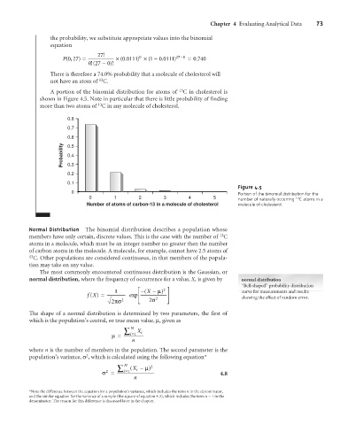
A portion of the binomial distribution for atoms of C in cholesterol is
shown in Figure 4.5. Note in particular that there is little probability of finding
13
more than two atoms of C in any molecule of cholesterol.
0.8
0.7
0.6
Probability 0.5

0.4
0.3
0.2
0.1
Figure 4.5
0 Portion of the binomial distribution for the
0 1 2 3 4 5 number of naturally occurring C atoms in a
13
Number of atoms of carbon-13 in a molecule of cholesterol molecule of cholesterol.

Normal Distribution The binomial distribution describes a population whose
13
members have only certain, discrete values. This is the case with the number of C
atoms in a molecule, which must be an integer number no greater then the number
of carbon atoms in the molecule. A molecule, for example, cannot have 2.5 atoms of
13 C. Other populations are considered continuous, in that members of the popula-
tion may take on any value.
The most commonly encountered continuous distribution is the Gaussian, or
normal distribution, where the frequency of occurrence for a value, X, is given by normal distribution
“Bell-shaped” probability distribution
2
1 é ( - X -m ) ù curve for measurements and results
(
fX) = exp ê 2 ú showing the effect of random error.
2ps 2 ë 2s û
The shape of a normal distribution is determined by two parameters, the first of
which is the population’s central, or true mean value, m, given as
N
å X i
m= i = 1
n
where n is the number of members in the population. The second parameter is the
2
population’s variance, s , which is calculated using the following equation*
N 2
å (X i - m )
2
s = i = 1 4.8
n
*Note the difference between the equation for a population’s variance, which includes the term n in the denominator,
and the similar equation for the variance of a sample (the square of equation 4.3), which includes the term n – 1 in the
denominator. The reason for this difference is discussed later in the chapter.