Page 91 - Modern Analytical Chemistry

1400-CH04 9/8/99 3:54 PM Page 74

74 Modern Analytical Chemistry

(a)

(b)

f (x) (c)

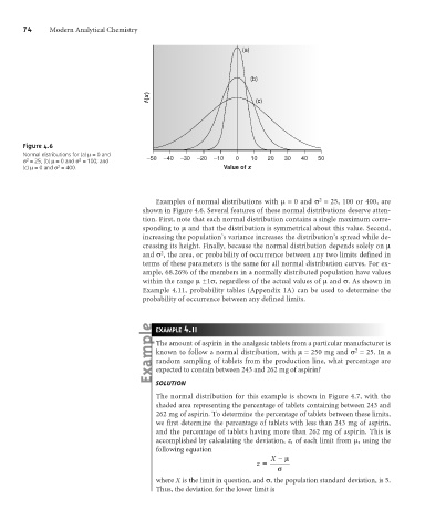
Figure 4.6
Normal distributions for (a) m= 0 and
2
2
s = 25; (b) m= 0 and s = 100; and –50 –40 –30 –20 –10 0 10 20 30 40 50
2
(c) m= 0 and s = 400. Value of x

2
Examples of normal distributions with m= 0 and s = 25, 100 or 400, are
shown in Figure 4.6. Several features of these normal distributions deserve atten-
tion. First, note that each normal distribution contains a single maximum corre-
sponding to mand that the distribution is symmetrical about this value. Second,
increasing the population’s variance increases the distribution’s spread while de-
creasing its height. Finally, because the normal distribution depends solely on m
2
and s , the area, or probability of occurrence between any two limits defined in
terms of these parameters is the same for all normal distribution curves. For ex-
ample, 68.26% of the members in a normally distributed population have values
within the range m±1s, regardless of the actual values of m and s. As shown in
Example 4.11, probability tables (Appendix 1A) can be used to determine the
probability of occurrence between any defined limits.

4
EXAMPLE .11
The amount of aspirin in the analgesic tablets from a particular manufacturer is
2
known to follow a normal distribution, with m= 250 mg and s = 25. In a
random sampling of tablets from the production line, what percentage are
expected to contain between 243 and 262 mg of aspirin?
SOLUTION

The normal distribution for this example is shown in Figure 4.7, with the
shaded area representing the percentage of tablets containing between 243 and
262 mg of aspirin. To determine the percentage of tablets between these limits,
we first determine the percentage of tablets with less than 243 mg of aspirin,
and the percentage of tablets having more than 262 mg of aspirin. This is
accomplished by calculating the deviation, z, of each limit from m, using the
following equation
X -m
z =
s
where X is the limit in question, and s, the population standard deviation, is 5.
Thus, the deviation for the lower limit is