Page 96 - Modern Analytical Chemistry

1400-CH04 9/8/99 3:54 PM Page 79

Chapter 4 Evaluating Analytical Data 79

25

20

15
Frequency 10

5

0
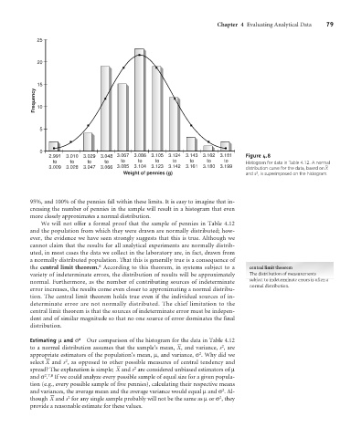
2.991 3.010 3.029 3.048 3.067 3.086 3.105 3.124 3.143 3.162 3.181 Figure 4.8
to to to to to to to to to to to Histogram for data in Table 4.12. A normal
3.009 3.028 3.047 3.066 3.085 3.104 3.123 3.142 3.161 3.180 3.199 distribution curve for the data, based on X –
Weight of pennies (g) and s , is superimposed on the histogram.
2

95%, and 100% of the pennies fall within these limits. It is easy to imagine that in-
creasing the number of pennies in the sample will result in a histogram that even
more closely approximates a normal distribution.
We will not offer a formal proof that the sample of pennies in Table 4.12
and the population from which they were drawn are normally distributed; how-
ever, the evidence we have seen strongly suggests that this is true. Although we
cannot claim that the results for all analytical experiments are normally distrib-
uted, in most cases the data we collect in the laboratory are, in fact, drawn from
a normally distributed population. That this is generally true is a consequence of
6
the central limit theorem. According to this theorem, in systems subject to a central limit theorem
variety of indeterminate errors, the distribution of results will be approximately The distribution of measurements
normal. Furthermore, as the number of contributing sources of indeterminate subject to indeterminate errors is often a
normal distribution.
error increases, the results come even closer to approximating a normal distribu-
tion. The central limit theorem holds true even if the individual sources of in-
determinate error are not normally distributed. The chief limitation to the
central limit theorem is that the sources of indeterminate error must be indepen-
dent and of similar magnitude so that no one source of error dominates the final
distribution.

Estimating mand s 2 Our comparison of the histogram for the data in Table 4.12
–
2
to a normal distribution assumes that the sample’s mean, X, and variance, s , are
2
appropriate estimators of the population’s mean, m, and variance, s . Why did we
–
2
select X and s , as opposed to other possible measures of central tendency and
–
2
spread? The explanation is simple; X and s are considered unbiased estimators of m
2 7,8
and s . If we could analyze every possible sample of equal size for a given popula-
tion (e.g., every possible sample of five pennies), calculating their respective means
2
and variances, the average mean and the average variance would equal mand s . Al-
–
2
2
though X and s for any single sample probably will not be the same as mor s , they
provide a reasonable estimate for these values.