Page 190 - Modern Control Systems

Chapter 3 State Variable Models

To write Equation (3.1) in terms of the state variables, we substitute the state variables
as already defined and obtain

dx 2
M— + bx 2 + kxi = u{t). (3.2)

Therefore, we can write the equations that describe the behavior of the spring-mass-
damper system as the set of two first-order differential equations

(3.3)
* 2
dt
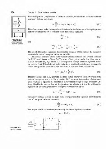
FIGURE 3.3
A spring-mass- and
damper system.
-b k 1
dx 2
M
77*2 _ 77*1 + 77 - (3.4)
dt M M M
This set of differential equations describes the behavior of the state of the system in
terms of the rate of change of each state variable.
As another example of the state variable characterization of a system, consider
the RLC circuit shown in Figure 3.4. The state of this system can be described by a set
of state variables {x h x 2), where x% is the capacitor voltage v c(t) and x 2 is the induc-
tor current i L{t). This choice of state variables is intuitively satisfactory because the
stored energy of the network can be described in terms of these variables as

1
Li i +|<v. (3.5)
Therefore X^IQ) and x 2(t 0) provide the total initial energy of the network and the
state of the system at t = t 0. For a passive RLC network, the number of state vari-
ables required is equal to the number of independent energy-storage elements. Uti-
lizing Kirchhoffs current law at the junction, we obtain a first-order differential
equation by describing the rate of change of capacitor voltage as

dv c
= C — = +u{t) - i L. (3.6)
r e
Kirchhoffs voltage law for the right-hand loop provides the equation describing the
rate of change of inductor current as

di L
-Ri L + v c. (3.7)
' dt
The output of this system is represented by the linear algebraic equation

= Ri L(t).
v 0

FIGURE 3.4
An RLC circuit.