Page 193 - Modern Control Systems

Section 3.3 The State Differential Equation 167
where y is the set of output signals expressed in column vector form. The state-space
representation (or state-variable representation) comprises the state differential
equation and the output equation.
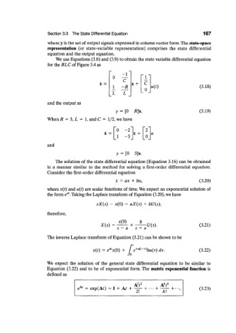
We use Equations (3.8) and (3.9) to obtain the state variable differential equation
for the RLC of Figure 3.4 as

- 1
0 —
C
x = x + C (3.18)
J_ -R 0 «(0
L L
and the output as
y = [0 R]x. (3.19)
When R = 3, L = 1, and C = 1/2, we have

"o -2~ V
x = 1 x +
L -3 J L°J
and

y = [0 3]x.
The solution of the state differential equation (Equation 3.16) can be obtained
in a manner similar to the method for solving a first-order differential equation.
Consider the first-order differential equation
x = ax + bu, (3.20)
where x(t) and u(t) are scalar functions of time. We expect an exponential solution of
at
the form e . Taking the Laplace transform of Equation (3.20), we have

sX{s) - x(0) = aX{s) + bU(s);
therefore,
x(0) b
X(s) = T ^ : + T^-tf(s). (3.21)
s — a s — a
The inverse Laplace transform of Equation (3.21) can be shown to be

at +a( T)
x{t) = e x(0) + [ e '- bu(T) dr. (3.22)
Jo
We expect the solution of the general state differential equation to be similar to
Equation (3.22) and to be of exponential form. The matrix exponential function is
defined as
k k
2,2 \ t
,A/ _ Mi + —— +•
= exp(Ar) = I + At + + (3.23)
2! k\