Page 195 - Modern Control Systems

Section 3.3 The State Differential Equation 169

-+• <? •*• p

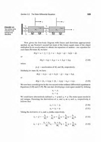
FIGURE 3.5 Cart 2 |A/VV
Two rolling carts M, M, Cart I •* • II
attached with
springs and
dampers. :0=331^=22=32:

Now, given the free-body diagram with forces and directions appropriately
applied, we use Newton's second law (sum of the forces equals mass of the object
multiplied by its acceleration) to obtain the equations of motion—one equation for
each mass. For mass Mj we have

Mip = « + / if + r f - « - k\{p ~ q) ~ bi{p - q),
/
or
Mi'p + b\p + k\p = u + k xq + b\q, (3.28)
where

p,q = acceleration of M\ and M 2, respectively.
we have
Similarly, for mass M 2
M 2q = k 1(p-q) + b r(p - q) - k 2q - b 2q,
or

M 2q + (ki + k 2)q + {b\ + b 2)q = k xp + b{p. (3.29)
We now have a model given by the two second-order ordinary differential equations in
Equations (3.28) and (3.29). We can start developing a state-space model by defining

*l = p,
x 2 = q.
We could have alternatively defined X\ = q and x 2 = P- The state-space model is
not unique. Denoting the derivatives of X\ and x 2 as x 3 and x 4, respectively, it
follows that
Xj = X, = p , (3.30)
x^ = x 2 — q. (3.31)

Taking the derivative of x 3 and x 4 yields, respectively,
b\ . k x 1 k± by .
(3.32)

k\ + k 2 b x + b 2 . k-y b\
(3.33)