Page 200 - Modern Control Systems

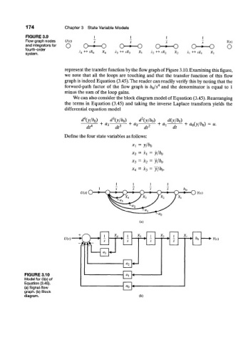
174 Chapter 3 State Variable Models
FIGURE 3.9
Row graph nodes U(s) s
and integrators for O o o o-*—o a O
fourth-order -o o
system. i 4 <-» sX 4 A'3 ^-^ .VA-j X^ A 2 <-» ,vX 2 X 2 i, <-» ,vX|

represent the transfer function by the flow graph of Figure 3.10. Examining this figure,
we note that all the loops are touching and that the transfer function of this flow
graph is indeed Equation (3.45). The reader can readily verify this by noting that the
forward-path factor of the flow graph is b$/s 4 and the denominator is equal to 1
minus the sum of the loop gains.
We can also consider the block diagram model of Equation (3.45). Rearranging
the terms in Equation (3.45) and taking the inverse Laplace transform yields the
differential equation model

2
d\y/b 0) M d\y/b Q) d (y/b 0) d(y/b 0)
^ —
dt 4 + a 3 dt- + a 2 dt —^— + rti—-— + a 0(y/b 0) = u.
l
dt
Define the four state variables as follows:
x\ = y/b 0
x 2 = ki = y/b 0
= = y/bo
x 3 x 2
XA = x 3 = y/bo.

U(s) O O ns)

(a)

n.v)

FIGURE 3.10
Model for G{s) of
Equation (3.45).
(a) Signal-flow
graph, (b) Block
diagram. (b)