Page 204 - Modern Control Systems

178 Chapter 3 State Variable Models
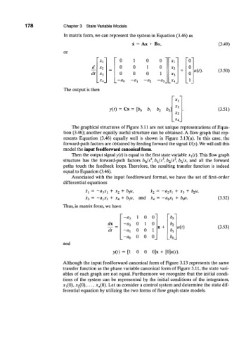
In matrix form, we can represent the system in Equation (3.46) as

x = Ax + BM, (3.49)
or
0 1 0 0 ~o~
* i X\
0 0 1 0 0
d x 2 x 2
+ u(t). (3.50)
dt 0 0 0 1 0
*3 *3
X4 -«() - « 1 -a 2 - « 3 |_X 4 _ _1_
The output is then

y(t) = Cx= [bo b x b 2 b 3] x 2 (3.51)
X3
x 4
The graphical structures of Figure 3.11 are not unique representations of Equa-
tion (3.46); another equally useful structure can be obtained. A flow graph that rep-
resents Equation (3.46) equally well is shown in Figure 3.13(a). In this case, the
forward-path factors are obtained by feeding forward the signal U($). We will call this
model the input feedforward canonical form.
Then the output signal y(t) is equal to the first state variable Xi(t). This flow graph
3
2
4
structure has the forward-path factors 6 0 A > bi/s , b 2/s , b 3/s, and all the forward
paths touch the feedback loops. Therefore, the resulting transfer function is indeed
equal to Equation (3.46).
Associated with the input feedforward format, we have the set of first-order
differential equations
Xi = -a^Xi + x 2 + b$u, x 2 = —a 2X[ + X3 + b 2u,
X3 = — a^X] + x 4 + biit, andX4 = — fl 0x 1 + b Qu. (3.52)
Thus, in matrix form, we have

1 0 (f
«3 bi
dx «2 0 1 0 x + b 2 u(t) (3.53)
dt 0 0 1 by
a Q 0 0 0_ bo
and
y(t) = [1 0 0 0]x + [0]M(0-

Although the input feedforward canonical form of Figure 3.13 represents the same
transfer function as the phase variable canonical form of Figure 3.11, the state vari-
ables of each graph are not equal. Furthermore we recognize that the initial condi-
tions of the system can be represented by the initial conditions of the integrators,
x
\(0), x 2 (0),..., x„(0). Let us consider a control system and determine the state dif-
ferential equation by utilizing the two forms of flow graph state models.