Page 207 - Modern Control Systems

Section 3.4 Signal-Flow Graph and Block Diagram Models 181

(a)

U{s) • ns)

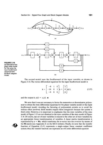
FIGURE 3.16
(a) Alternative flow
graph state model
for T(s) using the
input feedforward
canonical form.
{b) Block diagram
model. (b)

The second model uses the feedforward of the input variable, as shown in
Figure 3.16. The vector differential equation for the input feedforward model is

- 8 1 0" ~2~
-16 0 1 x + 8 u{t\ (3.57)
-6 0 0_ _6_

and the output is y(t) = *i(0- •

We note that it was not necessary to factor the numerator or denominator polyno-
mial to obtain the state differential equations for the phase variable model or the input
feedforward model. Avoiding the factoring of polynomials permits us to avoid the
tedious effort involved. Both models require three integrators because the system is
third order. However, it is important to emphasize that the state variables of the state
model of Figure 3.15 are not identical to the state variables of the state model of Figure
3.16. Of course, one set of state variables is related to the other set of state variables by
an appropriate linear transformation of variables. A linear matrix transformation is
represented by z = Mx, which transforms the x-vector into the z-vector by means of
the M matrix (see Appendix E on the MCS website). Finally, we note that the transfer
function of Equation (3.41) represents a single-output linear constant coefficient
system; thus, the transfer function can represent an «th-order differential equation