Page 210 - Modern Control Systems

184 Chapter 3 State Variable Models

>
l
Ms) Y(.s) R(s) - — • 10

2

(a) (b)
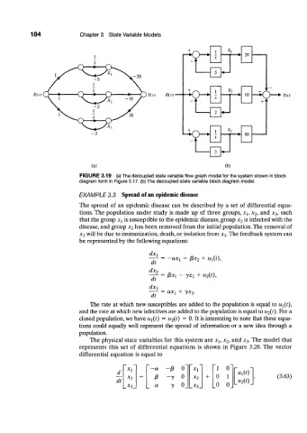
FIGURE 3.19 (a) The decoupled state variable flow graph model for the system shown in block
diagram form in Figure 3.17. (b) The decoupled state variable block diagram model.

EXAMPLE 3.3 Spread of an epidemic disease
The spread of an epidemic disease can be described by a set of differential equa-
tions. The population under study is made up of three groups, x h x 2, and x 3, such
is infected with the
that the group x± is susceptible to the epidemic disease, group x 2
disease, and group x 3 has been removed from the initial population. The removal of
x 3 will be due to immunization, death, or isolation from jq. The feedback system can
be represented by the following equations:

dxi
= —axi - /3*2 + «i(0i
dt
dx 2
= 0*! - yx 2 + K 2(0*
dt
dx 3
+ yx 2.
ax {
dt
The rate at which new susceptibles are added to the population is equal to U\(t),
and the rate at which new infectives are added to the population is equal to u 2(t). For a
closed population, we have u\(t) = u 2{t) = 0. It is interesting to note that these equa-
tions could equally well represent the spread of information or a new idea through a
population.
The physical state variables for this system are x u x 2, and x 3. The model that
represents this set of differential equations is shown in Figure 3.20. The vector
differential equation is equal to

* i —a -)8 0 Xl 1 0
d «i(0
*2 — -y 0 *2 + 0 1 (3.63)
dt "2(0
x a 0 0 0
, 3 y _ * 3 _