Page 208 - Modern Control Systems

182 Chapter 3 State Variable Models
n l
d"y d ' y d"'u /w-l,
a
dtn + n-l dtn- X + ••• + a 0y(t) = — + 6 m_, m-\ + + b 0u(t). (3.58)
dt
Accordingly, we can obtain the n first-order equations for the «th-order differential
equation by utilizing the phase variable model or the input feedforward model of this
section.

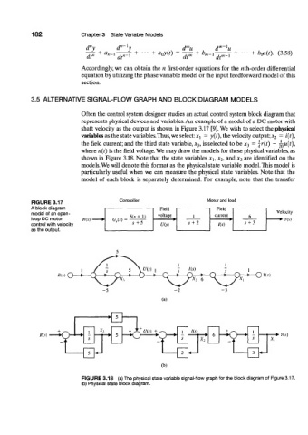
3.5 ALTERNATIVE SIGNAL-FLOW GRAPH AND BLOCK DIAGRAM MODELS

Often the control system designer studies an actual control system block diagram that
represents physical devices and variables. An example of a model of a DC motor with
shaft velocity as the output is shown in Figure 3.17 [9]. We wish to select the physical
variables as the state variables.Thus, we select: jq = y(t), the velocity output; x 2 = i(t),
= ^r(t) — ^u(t),
the field current; and the third state variable, x 3, is selected to be * 3
where u(t) is the field voltage. We may draw the models for these physical variables, as
x 2, and x 3 are identified on the
shown in Figure 3.18. Note that the state variables x h
models. We will denote this format as the physical state variable model. This model is
particularly useful when we can measure the physical state variables. Note that the
model of each block is separately determined. For example, note that the transfer

Controller Motor and load
FIGURE 3.17
A block diagram Field Meld
model of an open- voltage l current Velocity
+ ,)
loop DC motor R(s) cw-* , 6 m W 1 (Ji)
control with velocity U{s) s + 2 Ks) s + 3
as the output. s + 5

*<•*> O—>• O Ks)

(a)

5

+ /~N 1 h J U(s) + ~> lis) 1
m.t) s 5 fc 6 .V
_ J i •L X 2 i *.
5 2 <— 3
(b)

FIGURE 3.18 (a) The physical state variable signal-flow graph for the block diagram of Figure 3.17.
(b) Physical state block diagram.