Page 206 - Modern Control Systems

180 Chapter 3 State Variable Models

Multiplying the numerator and denominator by s~\ we have
l 2 3
Y(s) 2s~ + Ss~ + 6s~
T(s) = l 2 (3.54)
U(s) 1 + 8s~ + 16s~ + 6sr
-.
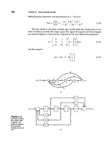
The first model is the phase variable state model using the feedforward of the
state variables to provide the output signal. The signal-flow graph and block diagram
are shown in Figures 3.15(a) and (b), respectively. The state differential equation is

0 1 0 0
0 0 1 x + 0 "(0, (3.55)
- 6 -16 - 8 1

and the output is

* i
v(0 = [6 8 2] (3.56)

U(s) O

(a)

U(s)

FIGURE 3.15
(a) Phase variable
flow graph state
model for T{s).
(b) Block diagram
for the phase
variable canonical
form. (b)