Page 197 - Modern Control Systems

Section 3.4 Signal-Flow Graph and Block Diagram Models 171
10

- 5
2 3
Time (s)

1 — ;
£
n
•3 0

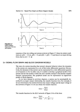
FIGURE 3.7
Initial condition
response of the two 2 3
cart system. Time (s)

response of the two rolling cart system is shown in Figure 3.7 when the initial condi-
tions are /?(0) = 10 cm, q(0) = 0, and p(0) = q(Q) = 0 and there is no input driving
force, that is, u{t) — 0. •

3.4 SIGNAL-FLOW GRAPH AND BLOCK DIAGRAM MODELS

The state of a system describes that system's dynamic behavior where the dynamics
of the system are represented by a set of first-order differential equations. Alterna-
tively, the dynamics of the system can be represented by a state differential equation
as in Equation (3.16). In either case, it is useful to develop a graphical model of the
system and use this model to relate the state variable concept to the familiar transfer
function representation. The graphical model can be represented via signal-flow
graphs or block diagrams.
As we have learned in previous chapters, a system can be meaningfully de-
scribed by an input-output relationship, the transfer function G(s). For example, if
we are interested in the relation between the output voltage and the input voltage of
the network of Figure 3.4, we can obtain the transfer function

G(s) =
U(sY

The transfer function for the RLC network of Figure 3.4 is of the form
V 0 (J)
G(s) = 2 (3.36)
U(s) s + ps + y