Page 198 - Modern Control Systems

172 Chapter 3 State Variable Models
where a, /3, and y are functions of the circuit parameters R, L, and Q respectively.
The values of a, /3, and y can be determined from the differential equations that
describe the circuit. For the RLC circuit (see Equations 3.8 and 3.9), we have
1 1 , ,
(3.37)

R
* 2 Xi ~X2, (3.38)
and
Rx 2. (3.39)

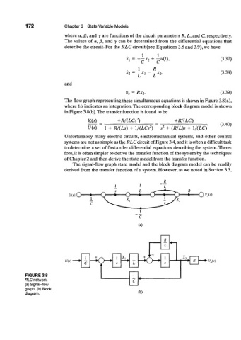
The flow graph representing these simultaneous equations is shown in Figure 3.8(a),
where 1/s indicates an integration. The corresponding block diagram model is shown
in Figure 3.8(b). The transfer function is found to be
2
+R/(LCs ) +R/(LC)
VQ(S) = = (3.40)
2
U(s) 1 + R/{Ls) + \/{LCs ) s 2 + (R/L)s + \/{LC)
Unfortunately many electric circuits, electromechanical systems, and other control
systems are not as simple as the RLC circuit of Figure 3.4, and it is often a difficult task
to determine a set of first-order differential equations describing the system. There-
fore, it is often simpler to derive the transfer function of the system by the techniques
of Chapter 2 and then derive the state model from the transfer function.
The signal-flow graph state model and the block diagram model can be readily
derived from the transfer function of a system. However, as we noted in Section 3.3,

U[s) O O w

(a)

R
L

, i t~
I X[ 1 + ,K I X-,
U(s) > R V„(.v)
s L .V
l
FIGURE 3.8 1
RLC network, C
(a) Signal-flow
graph, (b) Block
diagram. (b)