Page 270 - Modern Control Systems

244 Chapter 4 Feedback Control System Characteristics

•
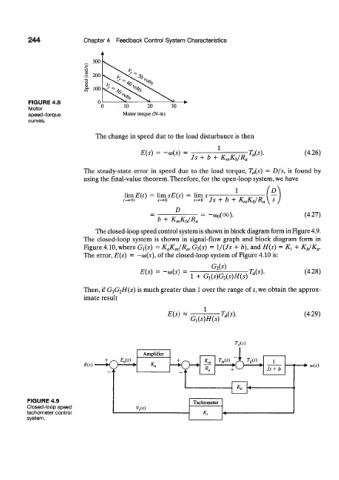
300
•3 V . /-
S 200 ^ X«%,,
eed />
CO 100 vf ^
FIGURE 4.8 0 ^ — •
Motor 10 20 30
speed-torque Motor torque (N-m)
curves.

The change in speed due to the load disturbance is then

1
£"(5) = -co(s) = Us). (4.26)
Js + b + K mK b/R a
The steady-state error in speed due to the load torque, T<i(s) = D/s, is found by
using the final-value theorem. Therefore, for the open-loop system, we have

1 D
\im E(t) = musECs) = lim s— : „ „ ,„ —
v
,-,00 ' ,_»o v } *-o Js + b \ s
D + K mK b/R a
= -wo(oo). (4.27)
b + K mK b/R a
The closed-loop speed control system is shown in block diagram form in Figure 4.9.
The closed-loop system is shown in signal-flow graph and block diagram form in
Figure 4.10, where G x(s) = K aK m/R a, G 2(s) = 1/(/5 + b), and H(s) = K t + K b/K a.
The error, E(s) = —<o(s), of the closed-loop system of Figure 4.10 is:
G 2(s)
E(s) = -<o(s) = Us)- (4.28)
1 + G l(s)G 2(s)H(s)
Then, if GiG 2H(s) is much greater than 1 over the range of s, we obtain the approx-
imate result

E(s)* Us). (4.29)
G^His)

TM)

+ ^ EjLs)
R(s) + 0 +> (O(S)

FIGURE 4.9
Closed-loop speed
tachometer control
system.