Page 80 - Modern Control Systems

54 Chapter 2 Mathematical Models of Systems

v(t)
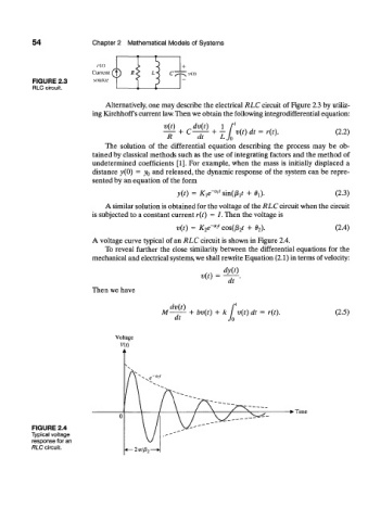
FIGURE 2.3
RLC circuit.

Alternatively, one may describe the electrical RLC circuit of Figure 2.3 by utiliz-
ing Kirchhoff s current law. Then we obtain the following integrodifferential equation:
t<0 dv(t) v
+ C dt il (t) dt = r(t). (2.2)
+
R
The solution of the differential equation describing the process may be ob-
tained by classical methods such as the use of integrating factors and the method of
undetermined coefficients [1]. For example, when the mass is initially displaced a
distance v(0) = y 0 and released, the dynamic response of the system can be repre-
sented by an equation of the form
v(0 = K^-"* s i n ^ ? + 0j). (2.3)

A similar solution is obtained for the voltage of the RLC circuit when the circuit
is subjected to a constant current r(t) = I. Then the voltage is
v(t) = K 2e-^ cos(/3 2r + S 2). (2.4)

A voltage curve typical of an RLC circuit is shown in Figure 2.4.
To reveal further the close similarity between the differential equations for the
mechanical and electrical systems, we shall rewrite Equation (2.1) in terms of velocity:
dy(t)
v(t) =
dt
Then we have

dv(t) f l
M — — + bv(t) + k I v(t) dt = r(t). (2.5)
dt Jo

• Time
FIGURE 2.4
Typical voltage
response for an
RLC circuit.