Page 83 - Modern Control Systems

Section 2.3 Linear Approximations of Physical Systems 57

a,

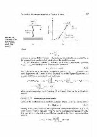
FIGURE 2.5
(a) A mass sitting
*• ) '
on a nonlinear
spring. (b)TTie
spring force (a)
versus y.
where

m dy
as shown in Figure 2.5(b). Thus, m = 2y G. A linear approximation is as accurate as
the assumption of small signals is applicable to the specific problem.
If the dependent variable y depends upon several excitation variables,
A,, x 2, • • •, x„, then the functional relationship is written as
y = g(xi, x 2,..., x n). (2.10)
The Taylor series expansion about the operating point x 1(), x 2() ,..., x lt is useful for a
linear approximation to the nonlinear function. When the higher-order terms are
neglected, the linear approximation is written as
dg (*, - * t()) + dg_
x
y = g(x h, x v — • >u) + ^ - (5x9 (x 2 -x 2 „) (2.11)
.1-=.(,,
H + \X n X n ) ,
dx„
where x 0 is the operating point. Example 2.1 will clearly illustrate the utility of this
method.

EXAMPLE 2.1 Pendulum oscillator model
Consider the pendulum oscillator shown in Figure 2.6(a). The torque on the mass is

T = MgL sin 9, (2.12)
where g is the gravity constant. The equilibrium condition for the mass is 6 0 = 0°.
The nonlinear relation between T and 6 is shown graphically in Figure 2.6(b).The
first derivative evaluated at equilibrium provides the linear approximation,
which is
dsin6
T - r 0 = MgL (9 - d 0).
M