Page 87 - Modern Control Systems

Section 2.4 The Laplace Transform 61

y«

O - X - - X -
-3 -2 -1
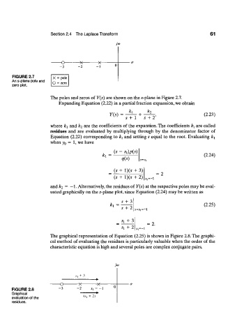
FIGURE 2.7 X = pole
An s-plane pole and
zero plot. O = zero

The poles and zeros of Y(s) are shown on the .s-plane in Figure 2.7.
Expanding Equation (2.22) in a partial fraction expansion, we obtain

Y{s) = + (2.23)
s + 1 5 + 2'
where k\ and k 2 are the coefficients of the expansion. The coefficients k t are called
residues and are evaluated by multiplying through by the denominator factor of
Equation (2.22) corresponding to k t and setting s equal to the root. Evaluating k±
when y 0 = 1, we have

(s - si)p(s)
fc = (2.24)
9(0 S = Sj

(s + l)(s + 3)
(s + l)(s + 2) S l =-i

and k 2 = — 1. Alternatively, the residues of Y(s) at the respective poles may be eval-
uated graphically on the .s-plane plot, since Equation (2.24) may be written as
s + 3
*i = (2.25)
s + 2 S = Si=— 1

+ 3
s t
= 2.
+ 2
5 X
*,=-!
The graphical representation of Equation (2.25) is shown in Figure 2.8. The graphi-
cal method of evaluating the residues is particularly valuable when the order of the
characteristic equation is high and several poles are complex conjugate pairs.

./<w

A, + 3
- O -x- X—
FIGURE 2.8 -2
Graphical
evaluation of the (.v, + 2)
residues.