Page 90 - Modern Control Systems

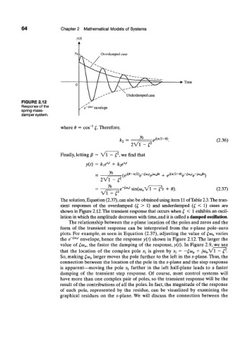
64 Chapter 2 Mathematical Models of Systems

• Time

Underdamped case
FIGURE 2.12
Response of the
spring-mass-
damper system.

where 6 = cos l £. Therefore,

yo :eJ(ir/2-0)
ko = (2.36)
2V1 - ('
2
Finally, letting p = V l - £ , we find that
1
y{t) = k^ ' + k 2e^
yo ( eiifi-TTi2) e-c^ ej^,fit + e/(V2-0) e-w e-M,/3r\
2V1 - i 1
yo fw 2
6).
+
.
v~„
r = :e- '''sin(ft> nVl . - £ f - • - , . (2.37)
,
viw 2
The solution, Equation (2.37), can also be obtained using item 11 of Table 2.3. The tran-
sient responses of the overdamped (£ > 1) and underdamped (£ < 1) cases are
shown in Figure 2.12. The transient response that occurs when t, < 1 exhibits an oscil-
lation in which the amplitude decreases with time, and it is called a damped oscillation.
The relationship between the s-plane location of the poles and zeros and the
form of the transient response can be interpreted from the s-plane pole-zero
plots. For example, as seen in Equation (2.37), adjusting the value of £G>„ varies
the e~^ J envelope, hence the response y(t) shown in Figure 2.12. The larger the
value of £,oi n, the faster the damping of the response, y(t). In Figure 2.9, we see
2
V
that the location of the complex pole ^ is given by s^ = —£o) n + j(o„ i - c .
So, making £a) n larger moves the pole further to the left in the 5-plane. Thus, the
connection between the location of the pole in the 5-plane and the step response
is apparent—moving the pole ^ farther in the left half-plane leads to a faster
damping of the transient step response. Of course, most control systems will
have more than one complex pair of poles, so the transient response will be the
result of the contributions of all the poles. In fact, the magnitude of the response
of each pole, represented by the residue, can be visualized by examining the
graphical residues on the s-plane. We will discuss the connection between the