Page 94 - Modern Control Systems

68 Chapter 2 Mathematical Models of Systems

il =
Inverting ?
input node + N o n i n v e r t i n g -o Output node
i'i input node +
lh f, = 0
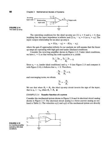
FIGURE 2.14
The ideal op-amp.

The operating conditions for the ideal op-amp are (1) i\ = 0 and i 2 = 0, thus
implying that the input impedance is infinite, and (2) v 2 — Vi = 0 (or Vi = ?^).The
input-output relationship for an ideal op-amp is
= - v^ = -K(vi - V2%
v Q K(v 2
o
where the gain K approaches infinity. In ur analysis, we will assume that the linear
op-amps are operating with high gain and under idealized conditions.
Consider the inverting amplifier shown in Figure 2.15. Under ideal conditions,
n
we have i^ = 0, so that writing the ode equation at v\ yields
Vl ~ ^in Vi v 0
= 0.
R^ R,
Since v 2 = V\ (under ideal conditions) and v 2 — 0 (see Figure 2.15 and compare it
with Figure 2.14), it follows that V\ = 0. Therefore,

R*
and rearranging terms, we obtain

vo_ ^ 2
^in R{
We see that when R 2 = R lf the ideal op-amp circuit inverts the sign of the input,
that is, v 0 = -v m when R 2 = R\. m

EXAMPLE 2.4 TVansfer function of a system
Consider the mechanical system shown in Figure 2.16 and its electrical circuit analog
shown in Figure 2.17. The electrical circuit analog is a force-current analog as out-
lined in Table 2.1. The velocities vi(t) and v 2(t) of the mechanical system are directly

R-,
V V V
«. i\ = 0
o V W ' 'l
+ T v 2 1^ -f
V W v
FIGURE 2.15 o
An inverting amplifier
operating with ideal
conditions.