Page 98 - Modern Control Systems

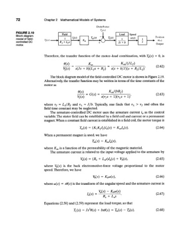
72 Chapter 2 Mathematical Models of Systems

Disturbance
FIGURE 2.19 Field Load
Block diagram Speed Position
model of field- \ l Us) ~X W l (o(s)
' ( v ) • > K m • m s)
controlled DC Rj + L fs *U • Js + b s Output
motor.

Therefore, the transfer function of the motor-load combination, with T d(s) = 0, is

6{s) K m KJ(JL f)
(2.62)
V f(s) s(Js + b){L fs + R f) s(s + b/J)(s + R f/L f)'

The block diagram model of the field-controlled DC motor is shown in Figure 2.19.
Alternatively, the transfer function may be written in terms of the time constants of the
motor as

K ml{bR f)
= G(s) = (2.63)
Vf(s) s{r fs + 1)(T LS + 1)'

where Tf = Lf/Rf and T L — J/b. Typically, one finds that T L > T f and often the
field time constant may be neglected.
The armature-controlled DC motor uses the armature current a as the control
i
variable. The stator field can be established by a field coil and current or a permanent
magnet. When a constant field current is established in a field coil, the motor torque is
T m(s) = (K.Kfl^Us) = KJ a(s). (2.64)

When a permanent magnet is used, we have
T m(s) = K mI a(s),

is a function of the permeability of the magnetic material.
where K m
The armature current is related to the input voltage applied to the armature by
V a(s) = (R a + L as)I a(s) + V h(s), (2.65)

where V h(s) is the back electromotive-force voltage proportional to the motor
speed. Therefore, we have

V b(s) = K ha>(s), (2.66)
where (o(s) - s6(s) is the transform of the angular speed and the armature current is

V a(s) - K,Ms)
(2.67)
+ L as
R a
Equations (2.58) and (2.59) represent the load torque, so that
2
T L(s) = Js 0{s) + bs0(s) = T m(s) - T d(s). (2.68)