Page 97 - Modern Control Systems

Section 2.5 The Transfer Function of Linear Systems 71

Armature
Stator
winding

Rotor windings
Brush

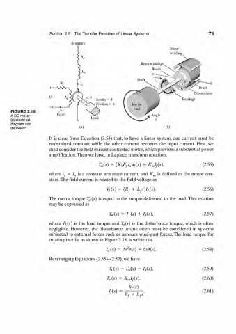
FIGURE 2.18
A DC motor Field
(a) electrical
diagram and
(b) sketch. (a) CM

It is clear from Equation (2.54) that, to have a linear system, one current must be
maintained constant while the other current becomes the input current. First, we
shall consider the field current controlled motor, which provides a substantial power
amplification. Then we have, in Laplace transform notation,
T m(s) = (K,K fI a)I f(s) = K ml f(s), (2.55)

where i a = /„ is a constant armature current, and K m is defined as the motor con-
stant. The field current is related to the field voltage as

V f(s) = (R f + L fs)I f(s). (2.56)

The motor torque T m(s) is equal to the torque delivered to the load. This relation
may be expressed as

TJs) = T L(s) + Us), (2.57)
where T/(s) is the load torque and T d(s) is the disturbance torque, which is often
negligible. However, the disturbance torque often must be considered in systems
subjected to external forces such as antenna wind-gust forces. The load torque for
rotating inertia, as shown in Figure 2.18, is written as
2
T L(s) = Js B(s) + bsd(s). (2.58)
Rearranging Equations (2.55)-(2.57), we have

T L(s) = TJs) - T d(s), (2.59)
TJs) = KJj{s\ (2.60)

V f{s)
I f(s) = (2.61)
R f + L fs'